What Is PID Tuning?
PID tuning is the process of adjusting the Proportional, Integral, and Derivative gains in a feedback control system to optimize response speed, minimize positioning errors, and eliminate oscillations or instability. PID controllers form the foundation of servo motor control, temperature regulation, process control, and countless automated systems requiring precise regulation of a measured variable against a setpoint.
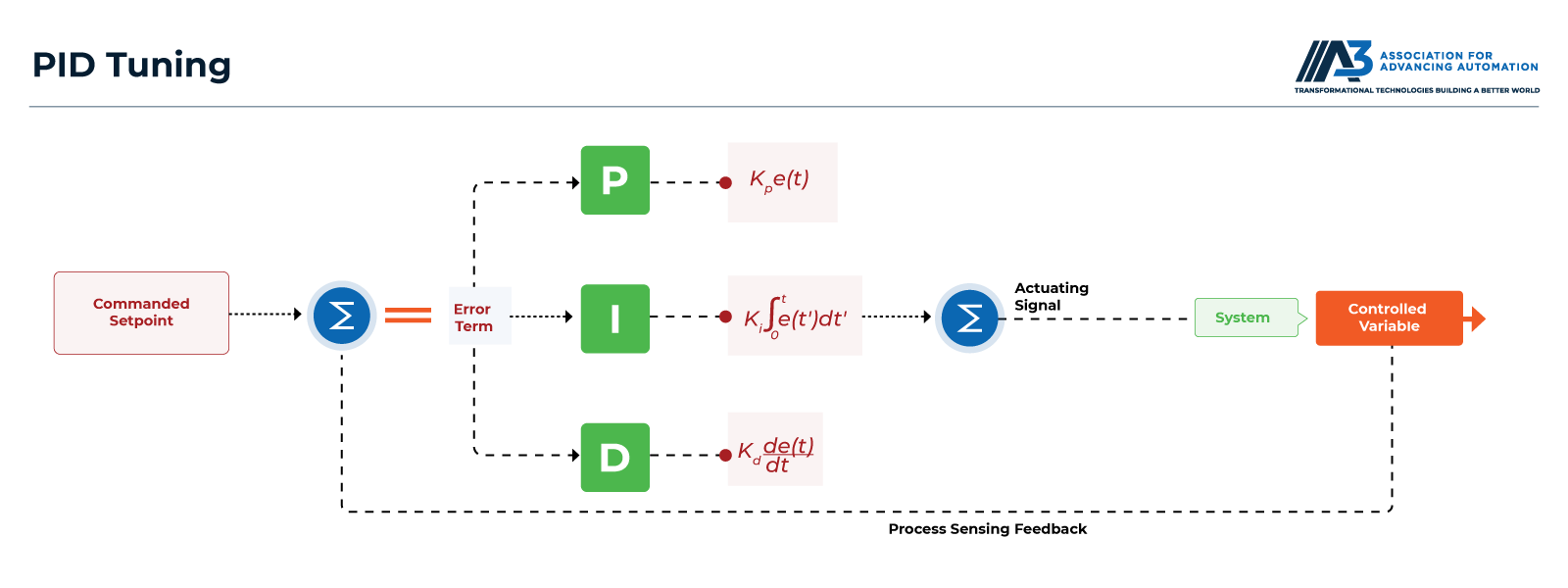
The acronym PID stands for the three control terms that work together to drive the system toward its target. The Proportional term responds to current error magnitude, the Integral term corrects accumulated error over time, and the Derivative term anticipates future error based on the rate of change. Proper tuning balances these three terms to achieve fast response without overshoot, stable operation without oscillation, and accurate positioning without steady-state error.
PID tuning directly impacts machine performance, cycle time, and product quality. Under-tuned systems move slowly and waste production time. Over-tuned systems oscillate, causing mechanical wear, positioning inaccuracy, and potential instability. Well-tuned systems reach target positions quickly and smoothly, maximizing throughput while maintaining accuracy and extending mechanical life.
What Do the P, I, and D Terms Do?
The Proportional term generates output proportional to current error magnitude, the Integral term corrects persistent steady-state errors by accumulating error over time, and the Derivative term dampens oscillations by responding to the rate of error change.
Proportional (P) Term
The P term multiplies current error by the proportional gain (Kp). If the position error is 5mm and Kp = 100, the proportional contribution is 500 units of drive signal. Larger errors produce stronger corrective action, while small errors generate gentle corrections. The P term provides the primary driving force toward the setpoint. Key characteristics:
- Fast initial response - Large errors immediately produce large corrections
- Proportional to distance - Correction force decreases as target approaches
- Steady-state error - Cannot eliminate final small errors alone
- Affects rise time - Higher Kp brings faster response but risks overshoot
A system with only P control settles near but not exactly at the setpoint. The remaining error, called steady-state error, persists because the small error generates insufficient drive force to overcome friction and complete the move.
Integral (I) Term
The I term accumulates error over time and multiplies this integral by the integral gain (Ki). If a 0.1mm error persists for 10 seconds, the integral term grows continuously, eventually generating enough output to eliminate the error. The I term specifically addresses steady-state errors that the P term cannot correct. Key characteristics:
- Eliminates steady-state error - Builds up force until error reaches zero
- Slow response - Takes time to accumulate sufficient correction
- Integral windup risk - Can overshoot if accumulated too much during large errors
- Affects settling time - Higher Ki eliminates error faster but may cause overshoot
Systems requiring exact positioning (no steady-state error acceptable) need I term contribution. However, excessive integral gain causes oscillation as the accumulated error continues driving past the setpoint before reversing.
Derivative (D) Term
The D term responds to the rate of error change, multiplying this derivative by the derivative gain (Kd). If error is decreasing rapidly (approaching setpoint quickly), the D term applies braking action to prevent overshoot. If error is increasing (moving away from setpoint), the D term adds corrective force. Key characteristics:
- Predicts future error - Anticipates where system is heading based on velocity
- Dampens oscillations - Applies braking when approaching setpoint too fast
- Sensitive to noise - Amplifies high-frequency sensor noise
- Affects overshoot - Higher Kd reduces overshoot and improves stability
The D term acts like shock absorbers in a car suspension, preventing bounce and oscillation. However, derivative action amplifies measurement noise since noise appears as rapid changes in the feedback signal. Excessive Kd causes jittery, noisy control outputs.
What Causes Overshoot and Instability?
Overshoot occurs when Proportional gain is too high relative to Derivative damping, causing the system to accelerate past the setpoint before corrective action can stop it, while instability results from excessive overall gain or Integral accumulation creating oscillations that amplify rather than decay.
Overshoot Mechanisms
Excessive P gain generates strong drive signals that accelerate the system rapidly toward the setpoint. Without sufficient D term damping, momentum carries the system past the target before deceleration can complete. The system then reverses, approaching from the opposite direction, potentially overshooting again and creating ringing - oscillations that gradually decay.
Insufficient D gain fails to apply adequate braking as the system approaches the setpoint. Even moderate P gains can cause overshoot when D term doesn't provide predictive damping. Increasing D gain reduces overshoot by applying stronger braking action proportional to approach velocity.
System inertia and delay - High-inertia loads or systems with transport delays (time between control output and observed effect) are particularly prone to overshoot. The control system commands deceleration, but the physical system continues moving due to inertia or the command hasn't yet affected the measured variable, causing overshoot before corrections take effect.
Instability and Oscillation
Positive feedback loops develop when overall gain is too high. The control system over-corrects errors, creating larger errors in the opposite direction, which generate even stronger over-corrections, producing oscillations that grow rather than decay. This instability can damage equipment and destroy product quality.
Integral windup occurs when large errors accumulate significant integral term contributions. Even after error crosses zero, the accumulated integral continues driving the system, causing overshoot. Modern controllers implement anti-windup mechanisms that limit integral accumulation or reset the integral when certain conditions occur.
Resonance excitation happens when control loop frequency matches mechanical resonances in the system. The controller inadvertently drives the system at its natural frequency, creating vibrations that amplify rather than diminish. This requires reducing gains or adding notch filters to suppress frequencies matching resonant modes.
Diagnosing Tuning Issues
Observing system response reveals tuning problems:
- Slow approach with no overshoot - P gain too low, increase Kp
- Fast response with significant overshoot - P gain too high or D gain too low, reduce Kp or increase Kd
- Continuous oscillation - Overall gain too high, reduce all terms proportionally
- Steady-state error remains - I gain too low or absent, increase Ki
- Oscillation that grows over time - System unstable, reduce gains significantly
What Is the Difference Between Manual and Auto-Tuning?
Manual tuning requires engineers to systematically adjust P, I, and D gains based on system response observation and tuning rules like Ziegler-Nichols, while auto-tuning uses algorithms that automatically inject test signals, measure system response, and calculate optimal gains without user intervention.
PID vs Auto-Tuning: Feature Comparison
Manual Tuning Process
Manual tuning typically follows systematic methods like Ziegler-Nichols or relay feedback approaches:
- Set I and D to zero, adjust only P gain
- Increase P until system oscillates at steady state (ultimate gain Ku)
- Measure oscillation period Tu
- Calculate initial gains based on formulas: Kp = 0.6×Ku, Ki = 1.2×Ku/Tu, Kd = 0.075×Ku×Tu
- Fine-tune based on response - adjust individual terms to optimize performance
Experienced engineers often skip formal methods and directly tune based on system response. They increase P until acceptable rise time is achieved, add D to eliminate overshoot, then introduce I to remove steady-state error, iterating until performance satisfies requirements.
Auto-Tuning Algorithms
Relay auto-tune induces controlled oscillations by switching the control output between two values while monitoring position. The system measures oscillation frequency and amplitude, then calculates gains using adaptive algorithms. This method is fast and works well for typical servo systems.
Step response auto-tune applies step inputs and analyzes the resulting position profile. The algorithm identifies system characteristics like time constants, delays, and gain, then calculates PID parameters matching desired response characteristics. This approach handles systems with significant delays or unusual dynamics.
Adaptive auto-tune continuously monitors system performance during normal operation, automatically adjusting gains to maintain optimal response as system characteristics change due to temperature, wear, or load variations. This advanced approach provides ongoing optimization without manual intervention.
When to Use Each Approach
Auto-tuning works well for:
- Standard servo systems with typical dynamics
- Multiple identical axes requiring consistent tuning
- Quick commissioning where "good enough" suffices
- Users without extensive control theory knowledge
Manual tuning is necessary for:
- Systems with unusual dynamics or multiple resonances
- Applications demanding maximum performance
- Situations where auto-tune creates instability or poor results
- Fine-tuning after auto-tune to optimize specific characteristics
Many engineers use auto-tune for initial setup, then manually fine-tune if performance improvements are needed. This hybrid approach combines auto-tune speed with manual optimization capability.
How Can Tuning Improve Throughput?
Proper PID tuning reduces move times by 20-50% through faster acceleration, shorter settling times, and elimination of oscillations that waste cycle time, directly increasing machine throughput without hardware modifications.
Cycle Time Components
A typical positioning move consists of:
- Acceleration phase - Motor accelerates load toward maximum velocity
- Constant velocity phase - Motor maintains target velocity during long moves
- Deceleration phase - Motor decelerates approaching target position
- Settling time - Residual oscillations decay until position error meets tolerance
Poor tuning extends settling time significantly. Under-tuned systems take 0.5-2 seconds to settle after a move that should complete in 0.2 seconds, wasting 0.3-1.8 seconds per cycle. On a pick-and-place system running 3,000 cycles per shift, this represents 15-90 minutes of lost production time daily.
Throughput Optimization Through Tuning
Aggressive acceleration - Higher P gains enable faster acceleration up to motor torque limits. Well-tuned systems reach maximum velocity 30-50% faster than conservative factory default tuning, reducing move time for short distances.
Reduced overshoot - Proper D term balance eliminates overshoot that would require reverse movement and settling. Each overshoot event adds 0.1-0.5 seconds to cycle time, compounding across thousands of cycles.
Faster settling - Optimized tuning reduces settling time from 0.5+ seconds to 0.05-0.1 seconds by eliminating oscillations and achieving critical damping. The system reaches and maintains position tolerance immediately rather than oscillating around the setpoint.
Higher velocity limits - Better tuning stability allows increasing maximum velocity limits without instability. Moves complete faster when the system can sustain higher speeds without control issues.
Real-World Performance Gains
A packaging machine with poorly tuned servos averaging 1.2 second cycles improved to 0.8 seconds per cycle after proper tuning, increasing throughput from 50 to 75 packages per minute (50% improvement) without hardware changes.
A CNC router with factory default tuning taking 45 minutes per part reduced to 32 minutes after aggressive tuning optimization that increased acceleration rates and reduced settling times while maintaining accuracy, improving throughput by 28%.
An assembly system with four poorly tuned axes showing settling oscillations improved from 90 units per hour to 130 units per hour (44% increase) through systematic tuning that eliminated settling time waste on each axis.
Conclusion
PID tuning optimizes feedback control systems by balancing Proportional response speed, Integral steady-state error correction, and Derivative damping to achieve fast, stable, accurate positioning. Understanding how P, I, and D terms affect system response enables diagnosing tuning problems and systematically improving performance.
The choice between manual and auto-tuning depends on application complexity, available expertise, and performance requirements. Auto-tuning provides quick commissioning and consistent results for standard systems, while manual tuning enables optimization for demanding applications or unusual dynamics. Many successful implementations combine auto-tune initial setup with manual fine-tuning for final optimization.
Proper tuning directly impacts production throughput by reducing move times, eliminating settling oscillations, and enabling higher acceleration and velocity limits. The investment in tuning optimization often delivers 20-50% throughput improvements without hardware costs, making PID tuning one of the most cost-effective performance enhancements available in motion control systems.
Recommended Resources
Explore additional materials to deepen your understanding of GigE Vision and related machine vision technologies
Automation's Unsung Hero: Why PID Control Still Matters in the Era of AI and IoT
Automation's Unsung Hero: Why PID Control Still Matters in the Era of AI and IoT.